Copyright David G. Green 1993.  Revised 1995.
This preprint may be copied and used provided that this
notice and the authorship details remain attached.
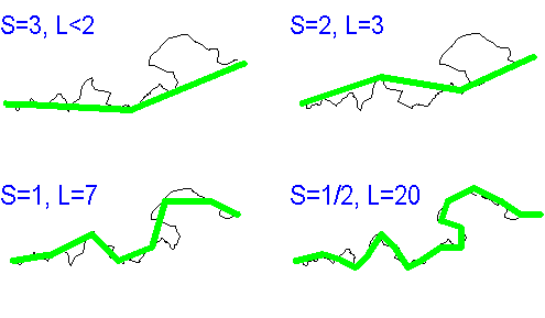
How long is the coast-line of Great Britain? At first sight this question may seem trivial. Given a map one can sit down with a ruler and soon come up with a value for the length. The problem is that repeating the operation with a larger scale map yields a greater estimate of the length (Fig. 1). If we actually went to the coast and measured them directly, then still greater estimates would result. It turns out that as the scale of measurement decreases the estimated length increases without limit. Thus, if the scale of the (hypothetical) measurements were to be infinitely small, then the estimated length would become infinitely large! Lewis Fry Richardson (quoted in Mandelbrot, 1983) noted this dependence of measured length to the measuring scale used.
In discussing measurement, scale can be characterized in terms of a measuring stick of a particular length: the finer the scale, the shorter the stick. Thus at any particular scale, we can think of a curve as being represented by a sequence of sticks (Fig. 1), all of the appropriate length, joined end-to-end. Clearly, any feature shorter than the stick will vanish from a map constructed in this way. Of course, no one actually makes maps by laying sticks on the ground, but the stick analogy reflects the sorts of distortions that are inevitably produced by the limited resolution of aerial photographs, by the length of survey transects, or by the thickness of the pens used in drafting. There is an analogy here, too, with the accuracy or frequency with which any sort of biological measurements are made.

Fig. 1  Using sticks of different size S to estimate the length L
        of a coastline.
The dependence of length (or area) measurements on scale poses great problems for biologists who need to use the results. For example, lakes that have a very convoluted shoreline are known to offer more area of shallows in relation to their total surface area, and thus support richer communities of plant and animal life. Attempts to characterize shore-line communities in terms of indexes that relate water surface to shoreline length have been frustrated by problems of scale.
Mandelbrot proposed the idea of a fractal (short for "fractional dimension") as a way to cope with problems of scale in the real world. He defined a fractal to be any curve or surface that is independent of scale. This property, referred to as self-similarity, means that any portion of the curve, if blown up in scale, would appear identical to the whole curve. Thus the transition from one scale to another can be represented as iterations of a scaling process (e.g. Fig. 2).

Fig. 2. Forming a cross by iteration of a simple procedure.
An important difference between fractal curves and the idealized curves that are normally applied to natural processes is that fractals are nowhere differentiable. That is, although they are continuous (smooth), they are "kinked" everywhere. Fractals can be characterized by the way in which representation of their structure changes with changing scale.
The notion of "fractional dimension" provides a way to measure how rough fractal curves are. We normally consider lines to have a dimension of 1, surfaces a dimension of 2 and solids a dimension of 3. However, a rough curve (say) wanders around on a surface; in the extreme it may be so rough that it effectively fills the surface on which it lies. Very convoluted surfaces, such as a tree's foliage or the internal surfaces of lungs, may effectively be three-dimensional structures. We can therefore think of roughness as an increase in dimension: a rough curve has a dimension between 1 and 2, and a rough surface has a dimension somewhere between 2 and 3. The dimension of a fractal curve is a number that characterizes the way in which the measured length between given points increases as scale decreases. Whilst the topological dimension of a line is always 1 and that of a surface always 2, the fractal dimension may be any real number between 1 and 2. The fractal dimension D is defined by
         log ( L2 / L1 )
     D = ---------------           ... (1)
         log ( S1 / S2 )
where L1, L2 are the measured lengths of the curves (in units), and S1, S2 are the sizes of the units (i.e. the scales) used in the measurements.
For the shoreline shown in Fig. 1, measurements for S=1 and S=1/2 give lengths of L=7 and L=20, respectively. So
D = log (20/7) / log (2) = 1.51
In similar fashion, the transition from S=1 to S=2 yields the slightly smaller estimate of D = 1.22 and from S=2 to S=3, D ~ 1.13.
It is important to realize that the above way of estimating fractal dimension applies only to certain sorts of data. Suppose that we wish to measure fractal properties of, say, the surface of a coral reef. There are two different sorts of measurements that we might make. One sort of measurement would consist of measuring distances between two points on the reef with measuring sticks of varying lengths (as in Fig. 1). Estimates of D for the reef surface would then be made using equation 1. If instead we moved along the same transect and measured, say, the height of the reef surface above the substrate, then we could not measure fractal index in the same way. For the height data we would have to estimate the fractal dimension from the power spectrum, or the variogram, of the data series. It turns out that if D is the fractal index, w is a frequency, and S(w) is the spectral value of w, then
     S(w) ~ k w^5 - 2D.            ... (2)


It is important to realize that true fractals are an idealization.
No curve or surface in the real world is a true fractal; real objects
are produced by processes that act over a finite range of scales only.
Thus estimates of D may vary with scale, as they do in the above
example. The variation can serve to characterize the relative importance
of different processes at particular scales. Mandelbrot called the breaks
between scales dominated by different processes "transition zones".
The idea of self-similarity means that if we shrink or enlarge a fractal pattern, its appearance should remain unchanged. Conversely, fractal patterns usually arise when simple patterns are transformed repetitively on smaller and smaller scales (e.g. Fig. 2). An important class of processes that produce fractal patterns are random iteration algorithms, which produce images of fractal objects. The procedure is akin to using a pen to mark dots at random on a sheet of paper. However, instead of being completely random, the movement of the pen from one position to the next is selected, at random, from a set of rules, each having fixed probability of being chosen. We can define these rules by affine transformations. An affine transformation A (in two dimensions) is a function that performs some combination of scaling, rotation, and translation on points in a plane and takes the general form
     Ax (x) = ax + by + e ,           ... (3)

     Ay (y) = cx + dy + f .
Table 1 summarizes the affine transformations associated with random iteration algorithms that produce pictures of ferns and grasses. For each transformation, the table lists the values of the parameters a, b, c, d, e, f in equation (2). The probability p assigns the frequency with which the transformation is used.
![]()
Fig. 3. A fractal fern.
Table 1 Affine transformations associated with some simple fractal images
------------------------------------------------------
Parameter* a      b      c     d      e     f      p
------------------------------------------------------
Fern      0.0    0.0    0.0   0.16   0.0   0.0   0.10
          0.2   -0.26   0.23  0.22   0.0   1.6   0.08
         -0.15   0.28   0.26  0.24   0.0   0.44  0.08
          0.75   0.04  -0.04  0.85   0.0   1.6   0.74

Grass     0.0    0.0    0.0   0.5    0.0   0.0   0.15
          0.02  -0.28   0.15  0.2    0.0   1.5   0.10
          0.02   0.28   0.15  0.2    0.0   1.5   0.10
          0.75   0.0    0.0   0.5    0.0   4.6   0.65
------------------------------------------------------

* See equation 3 for the meaning of the parameters.
Brownian Motion is an example of a process that has a fractal dimension of 2. It occurs in microscopic particles and is the result of random jostling by water molecules (if water is the medium). The path of such a particle is a "random walk" in which both direction and distance are uniformly distributed random variables. So in moving from a given location in space to any other, the path taken by the particle is almost certain to fill the whole space before it reaches the exact point that is the 'destination'.
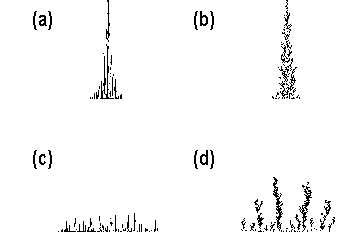
Another aspect of brownian motion is its effect on the formation of aggregates such as crystals. Figure 4 shows structures formed under different assumptions about the relative rate of horizontal movement (h) and the probability (p) of a settling particle sticking to fized particles as it brushes past. In the figure the following values are shown: (a) h=1, p=0; (b) h=1, p=1; (c) h=10, p=0; (d) h=10, p=1. "Sticky" particles (p=1 in the figure) tend to form structures resembling (say) trees or mosses. Such properties are exploited in animation to generate pictures of artificial plants and landscapes.

Fig. 4. Structures arising from brownian motion of falling particles.
The efficiency of the lungs in diffusing oxygen from the inhaled air is directly proportional to the surface available. So for a given volume of lung it is highly advantageous to maximize the surface area. The internal surfaces of lung tissues thus have extremely high fractal dimension (about 2.9).